

🕔 Estimated reading time: 32 minutes
The logic of Causal-Foliated Signaling
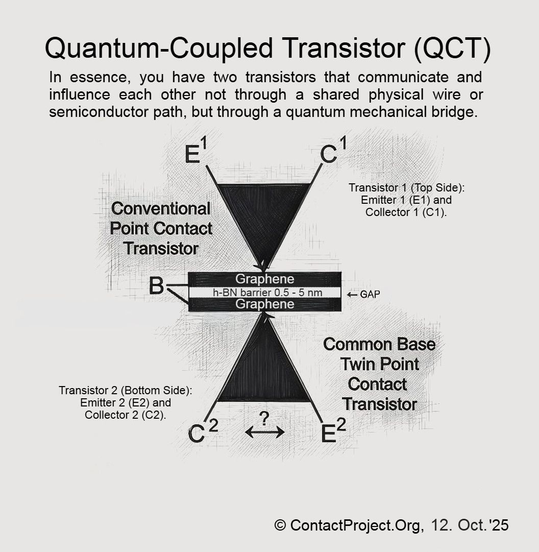
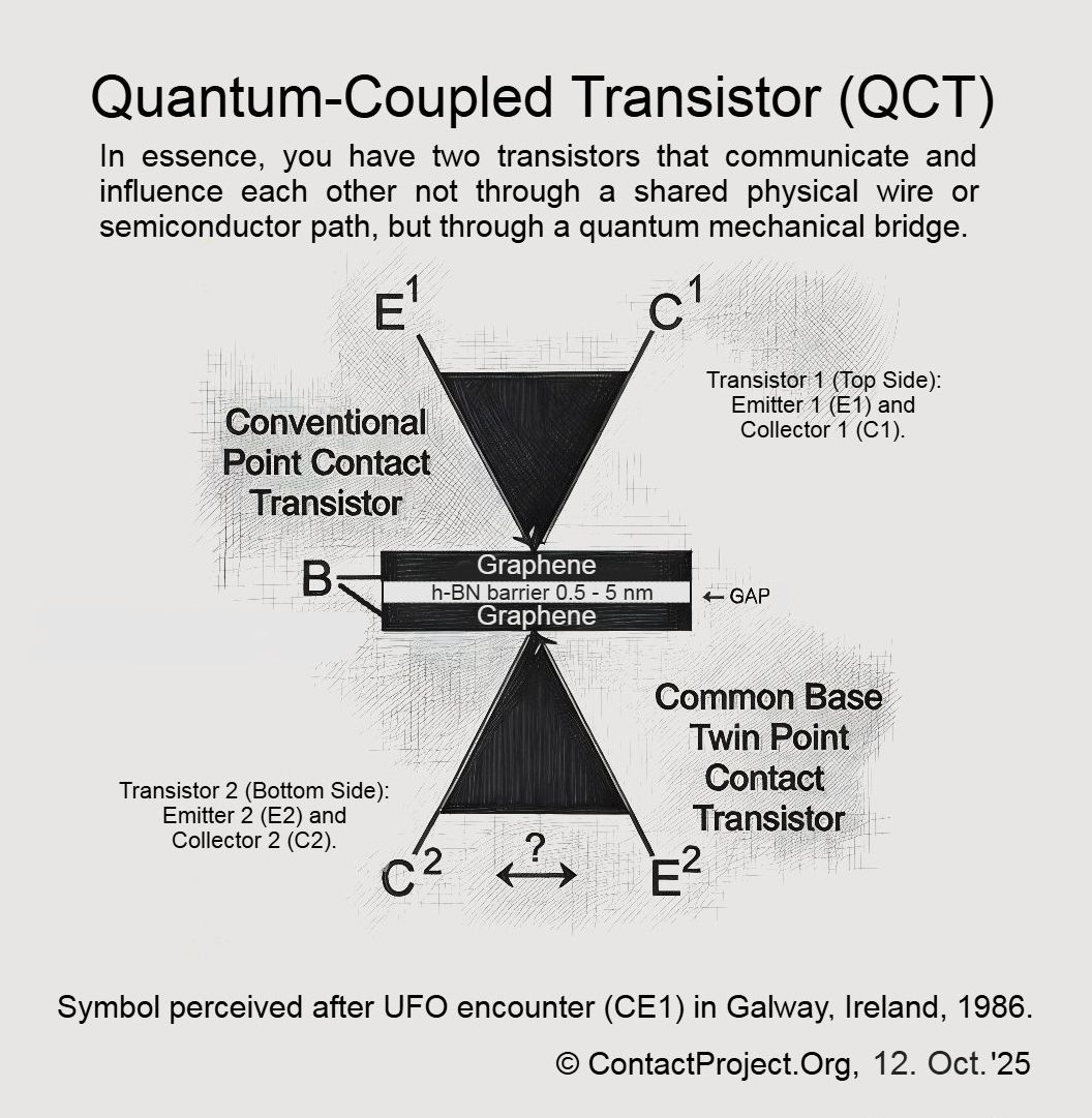
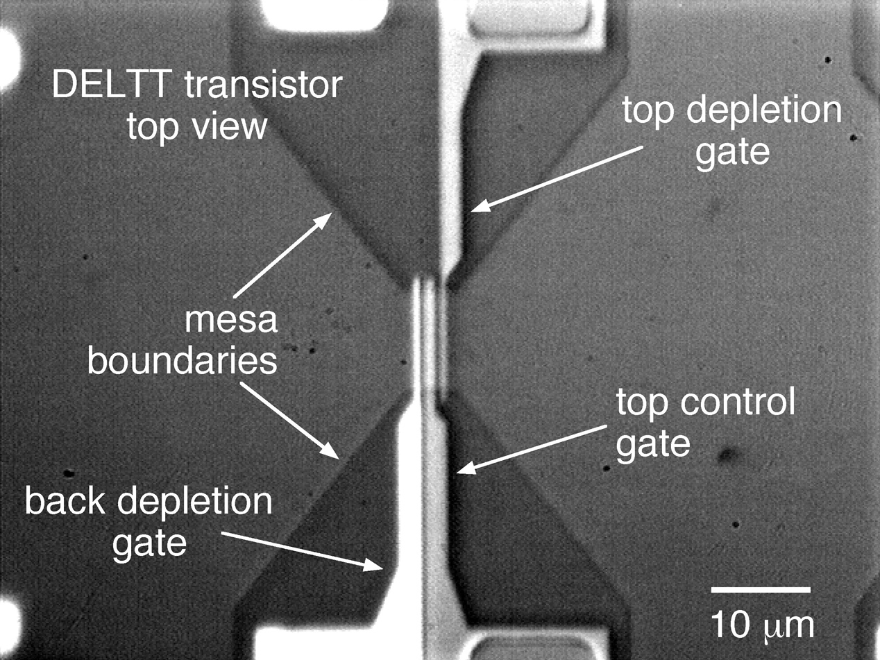
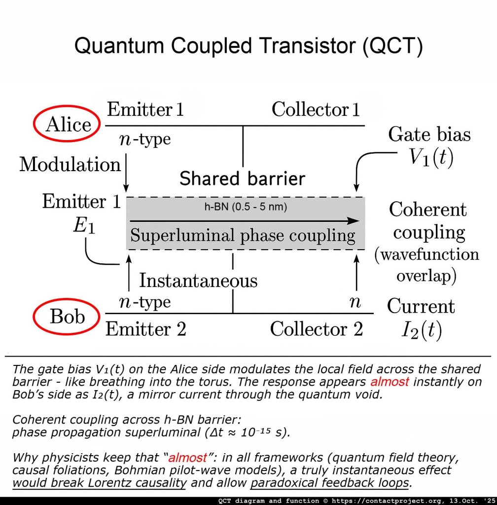
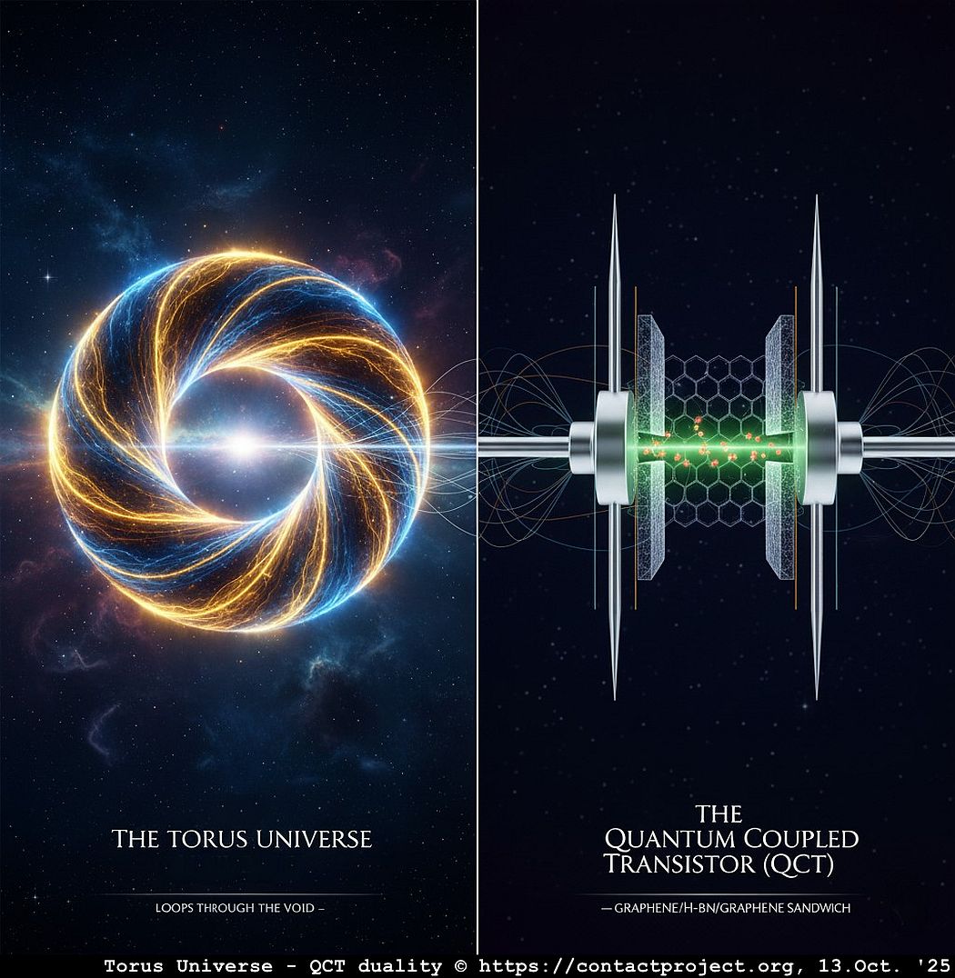
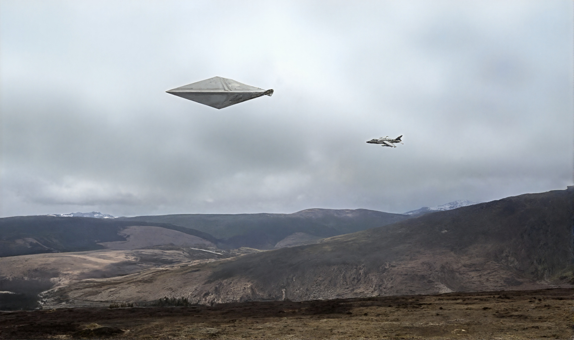
The theory of Causal-Foliated Signaling (CFS) proposes that time contains hidden layers that enable limited faster-than-light coherence between quantum systems. Researchers may soon be using the Quantum-Coupled Transistor (QCT) – a dual-graphene nanodevice – to test these effects directly and determine whether they can occur without breaking the known laws of physics.
At its heart, CFS asks a provocative question: What if certain kinds of waves, such as evanescent or near fields, can share phase information faster than light, yet still preserve causality?
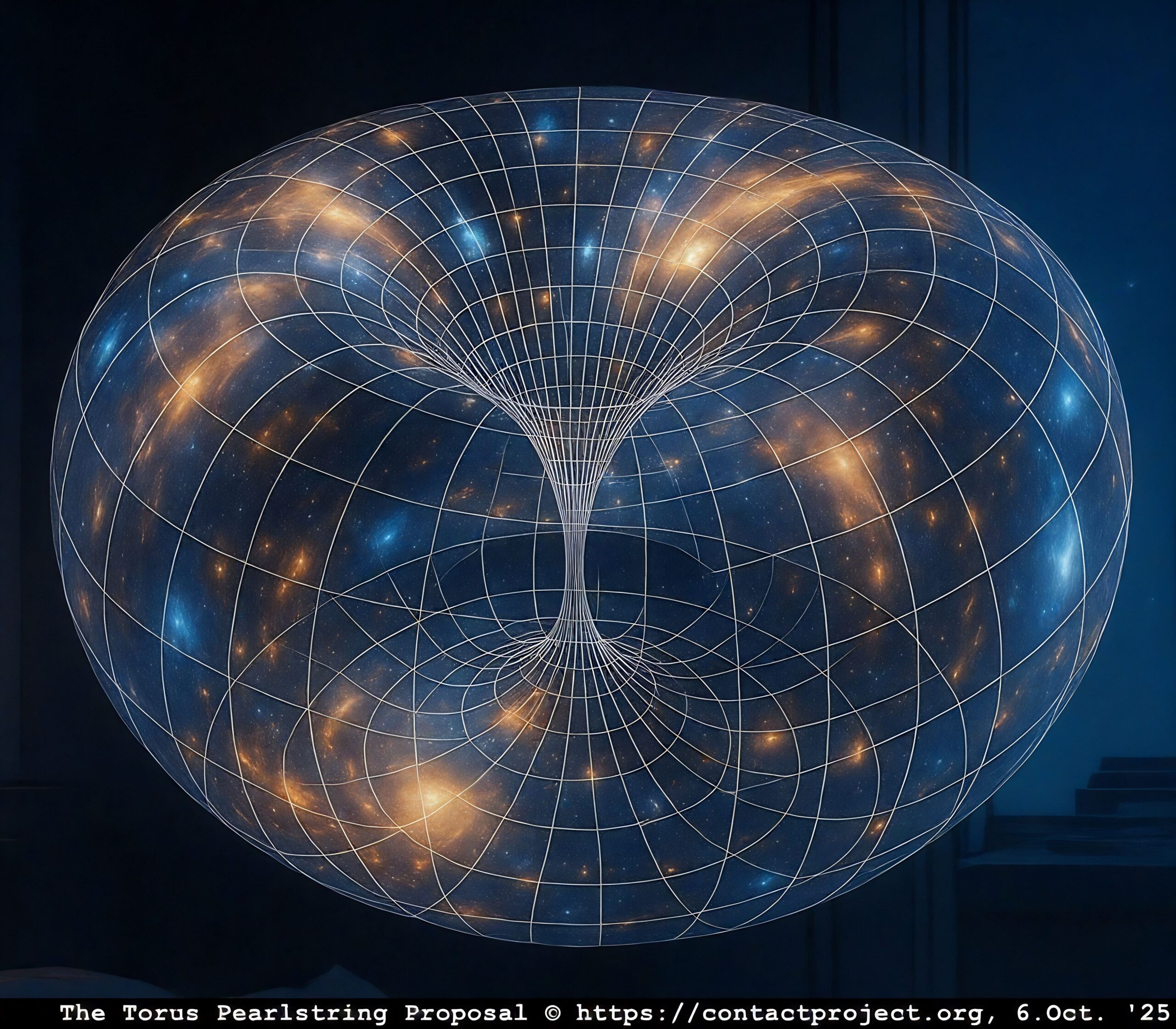
If so, spacetime might not be perfectly uniform. It could contain a subtle internal structure – a “layering” of time, where information moves slightly ahead within each layer while remaining consistent across the whole.

In this view, the universe unfolds like the pages of a vast cosmic book: each page turns in perfect order, even if some turn just a little faster than others. CFS offers a refined vision of relativity – one that permits structured superluminal coherence while keeping the story of cause and effect intact.
Part II. Causal-Foliated Signaling (CFS)
- Core Axioms
- Kinematics and Dynamics
- Quantum Rules and Conservation
- Experimental Predictions
- Test Protocols
- Role of the QCT
1. Core Axioms
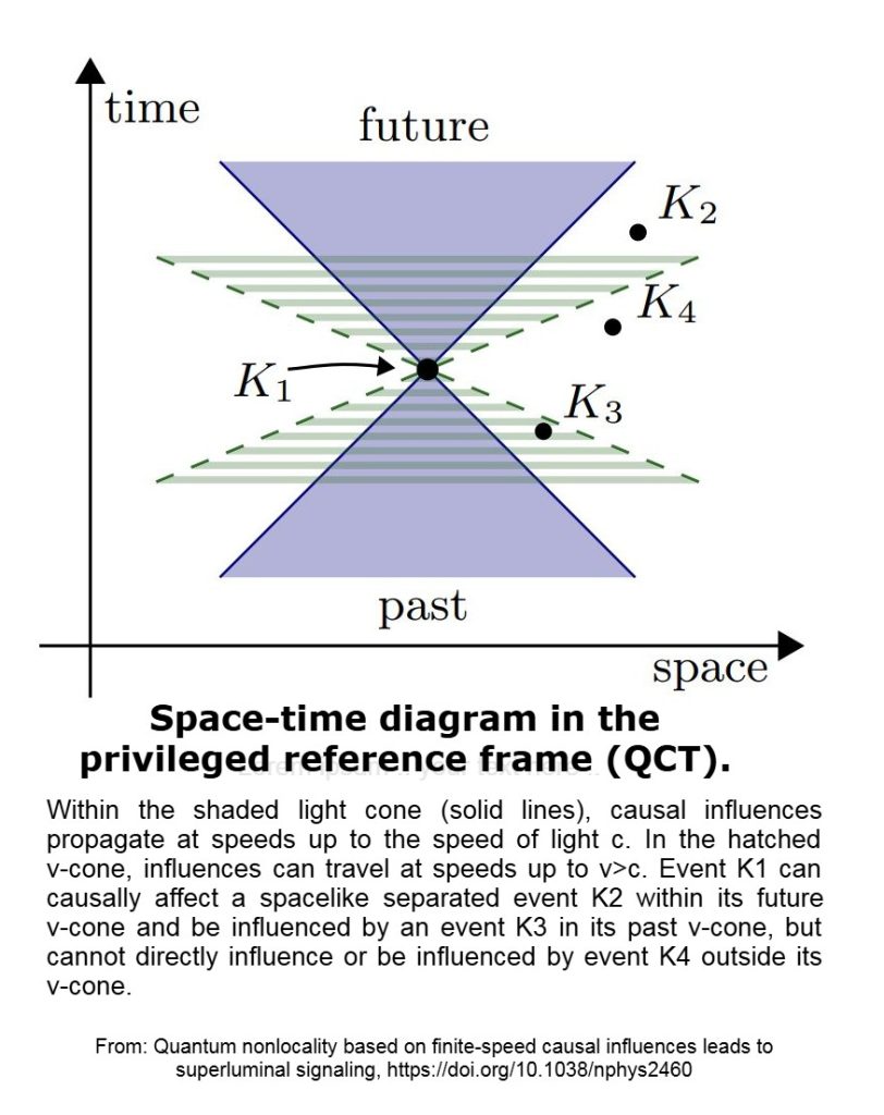
- Global Time Foliation: Spacetime possesses a preferred global slicing (cosmic time, defined by timelike vector uᵃ). All signals – luminal and superluminal – are ordered by this foliation.
- Enlarged Signal Cone: Beyond the light cone, a broader “signal cone” exists for specific media or fields (χ).
- Chronology Protection: Closed signal loops are dynamically forbidden by solvability constraints.
- Operational Locality: Standard experiments remain Lorentz-invariant; deviations occur only within enabled media.
2. Kinematics and Dynamics
- Preferred Frame: Aligned approximately with the CMB rest frame.
- Signal Field (χ): Couples weakly to EM carriers, widening the causal cone.
- Superluminal Characteristics: PDEs in enabled media exhibit propagation outside the g-lightcone.
- No-Loop Constraint: Integral conditions prevent time-decreasing causal loops.
3. Quantum Rules and Conservation
We built a tiny region (the QCT gap) where quantum near-fields can be gently shaped so that a barely detectable, faster-than-light pattern shows up in otherwise random data – small enough to keep physics safe, clear enough to test in the lab.
If the compact statement above makes sense to you, then you can expand the redlined Quantum Rules below by clicking on the black ▶ triangles, for a MORE detailed discussion.
For general readers, each section includes a brief explanation (without math) followed by an analogy. Although most people will never have heard of the no-communication theorem (prohibiting faster-than-light communication… by entanglement), it is placed prominently here because of its fundamental importance, and because a controlled relaxation of that rule is explored here.
[click to open] Relaxed No-Communication Theorem: In enabled media, nonlinear/post-selected dynamics allow tiny classical capacity > 0.
Claim (operational):
In an enabled medium (e.g., a QCT gap acting as χ-enabled near-field), a weak, localized nonlinearity or explicit post-selection can produce a small but finite classical capacity C>0 between spacelike-separated parties without violating global unitarity or the Born rule.
Setup
Let ρAB be a bipartite state shared by Alice and Bob. In standard QM with local CPTP maps and no post-selection, Bob’s reduced state is independent of Alice’s choice:
ρB′=TrA[(ΦA⊗IB)(ρAB)]=ρB, (no-signaling)
In an enabled QCT region, model Alice’s controlled operation as a weakly nonlinear perturbation of a CPTP map:
ΦA(V)(⋅)=ΛA(⋅)+ε\mathcal{N}_A^{(V)}[⋅], 0<ε≪1,[/latex] <p>where [latex]V is Alice’s control (e.g., interlayer bias), ΛA is CPTP and \mathcal{N}_A^{(V)} is a bounded nonlinear functional active only inside the χ-enabled medium.Bob’s state becomes
ρB′(V)=TrA[(ΦA(V)⊗IB)ρAB]=ρB(0)+εΔρB(V),with
ΔρB(V)=TrA [(NA(V)⊗IB)ρAB].\Delta\rho_B(V)=\mathrm{Tr}_A\!\Big[\big(\mathcal{N}_A^{(V)}\otimes \mathbb{I}_B\big)\rho_{AB}\Big].ΔρB(V)=TrA[(NA(V)⊗IB)ρAB].
If \Delta\rho_B(V_0)\neq \Delta\rho_B(V_1), then Bob’s outcome statistics depend (slightly) on Alice’s choice V, enabling classical communication at order \varepsilon.
For a POVM \{M_y\} on Bob, the detection probabilities are
P(y∣V)=Tr[MyρB′(V)]=P0(y)+εΔP(y∣V),ΔP(y∣V):=Tr[MyΔρB(V)].Capacity with weak signaling
Let Alice send a binary symbol X\in\{0,1\} by choosing V\in\{V_0,V_1\}.. Bob measures Y\in\{0,1\}. Define
\delta := P(Y=1\mid V_1)-P(Y=1\mid V_0)=\varepsilon\,\Delta P + O(\varepsilon^2),with baseline error probability p:=P(Y=1∣V0).
For a binary-input, binary-output channel in the small-signal limit ∣\delta|\ll 1, the Shannon capacity admits the quadratic approximation
C \;\approx\; \frac{\delta^2}{2\ln 2}\,\frac{1}{p(1-p)} \;+\; O(\delta^4), \qquad C>0\ \text{iff}\ \delta\neq 0.
Thus any nonzero \delta (hence any nonzero \varepsilon-order dependence on V) yields a finite C>0.
Role of post-selection
If Bob (or a joint coincidence circuit) post-selects on an outcome window W with success probability pW, the conditional state is
\rho_{B\!\mid W}(V)\;=\;\frac{\Pi_W\,\rho_B'(V)\,\Pi_W}{\mathrm{Tr}\!\big[\Pi_W\,\rho_B'(V)\big]}, \qquad \Pi_W=\Pi_W^\dagger=\Pi_W^2.Because of the normalization by \mathrm{Tr}[\Pi_W\rho_B'(V)], the mapping \rho'_B \mapsto \rho_B^{\mid W} is nonlinear, and the conditioned statistics can acquire a V-dependence even when the unconditioned no-signaling equality holds. In practice, post-selection scales the useful rate by pW:
C_{\mathrm{eff}} \approx p_W , C.Consistency conditions
To avoid global pathologies:
- Localization: \mathcal{N}_A^{(V)} is confined to the χ-enabled region (e.g., the QCT gap).
- Smallness: \varepsilon is sufficiently small to preserve stability and energy bounds.
- Global unitarity & Born rule: Ensemble dynamics remain CPTP; deviations (if any) are confined to the conditioned, local detector maps (post-selection) or to the weak-nonlinear sector inside the medium.
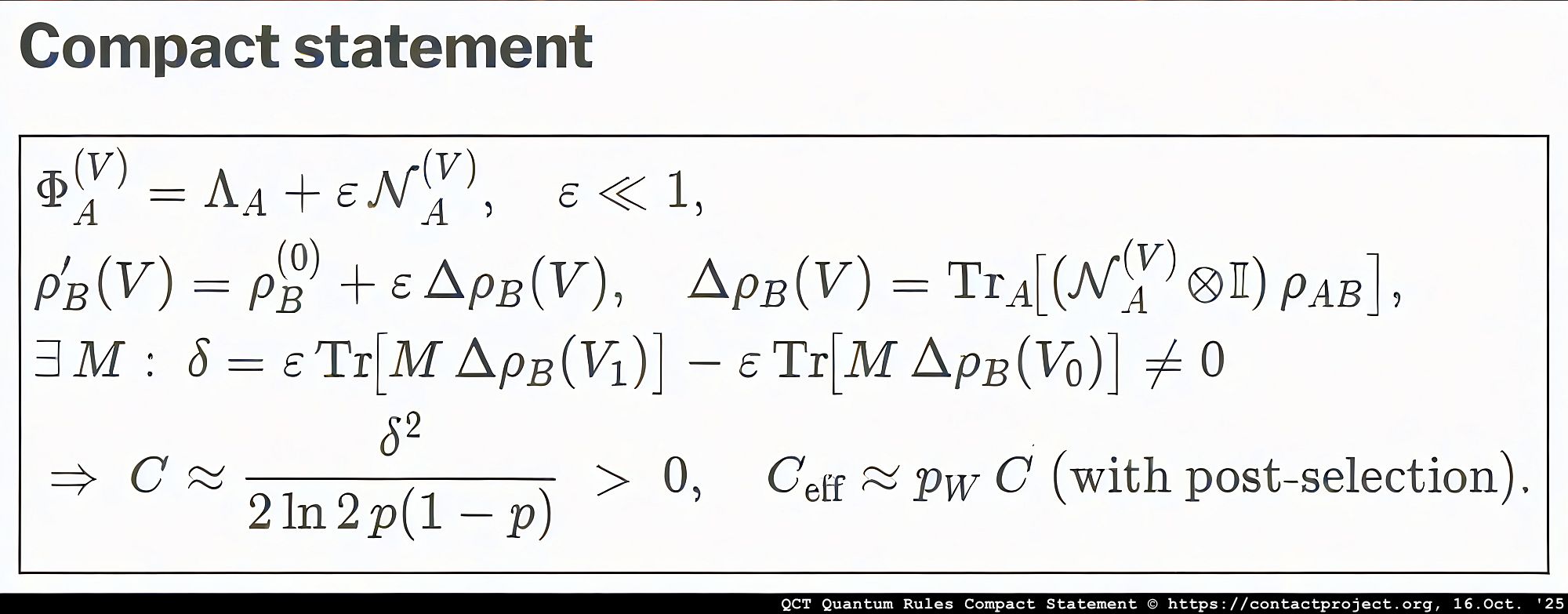
Compact statement
\boxed{ \begin{aligned} &\Phi_A^{(V)}=\Lambda_A+\varepsilon\,\mathcal{N}_A^{(V)},\quad \varepsilon\ll 1,\\ &\rho_B'(V)=\rho_B^{(0)}+\varepsilon\,\Delta\rho_B(V),\quad \Delta\rho_B(V)=\mathrm{Tr}_A\!\big[(\mathcal{N}_A^{(V)}\!\otimes\!\mathbb{I})\,\rho_{AB}\big],\\ &\exists\,M:\ \delta=\varepsilon\,\mathrm{Tr}\!\big[M\,\Delta\rho_B(V_1)\big]-\varepsilon\,\mathrm{Tr}\!\big[M\,\Delta\rho_B(V_0)\big]\neq 0 \\ &\Rightarrow\ C \approx \dfrac{\delta^2}{2\ln 2\, p(1-p)} \;>\;0,\quad C_{\text{eff}}\approx p_W\,C\ \text{(with post-selection)}. \end{aligned}}Here’s a breakdown and fact check of the compact mathematical statement:
The mathematical statement is a representation of a result in quantum information theory, related to the calculation of the capacity of a quantum channel with a small perturbation. It connects the physical description of a quantum channel to the resulting channel capacity, incorporating concepts like state perturbation, distinguishability of output states, and the effect of post-selection. Let's break down each part to verify its components:
Channel and State Perturbation
\Phi_A(V) = \Lambda_A + \epsilon N_A(V), \epsilon \ll 1: This describes a quantum channel \Phi_A acting on a system A. It consists of a dominant, constant part \Lambda_A and a small perturbation \epsilon N_A(V), where \epsilon is a small parameter and V is some controllable parameter of the channel. This is a standard way to represent a slightly modulated or noisy quantum channel. \rho_B'(V) = \rho_B(0) + \epsilon \Delta\rho_B(V): This shows the effect of the channel on part of a larger quantum state. It indicates that the output state of a subsystem B, \rho_B'(V), is a slightly perturbed version of an initial state \rho_B(0). The perturbation \Delta\rho_B(V) is proportional to the small parameter \epsilon. \Delta\rho_B(V) = Tr_A[(N_A(V) \otimes I)\rho_{AB}]: This is the explicit form of the first-order perturbation to the state of system B. It is derived by taking the partial trace (Tr_A) over system A of the action of the perturbative part of the channel on a larger, entangled state \rho_{AB}. This is a standard and correct application of the rules of quantum mechanics.
Distinguishability of States
\exists M: \delta = \epsilon Tr[M\Delta\rho_B(V_1)] - \epsilon Tr[M\Delta\rho_B(V_0)] \neq 0: This is the crucial step for establishing a non-zero channel capacity. It states that there exists a measurement operator (a Hermitian operator) M that can distinguish between the perturbed states corresponding to two different settings of the channel parameter, V_1 and V_0. The quantity \delta represents the difference in the expectation value of the measurement M for the two output states. The fact that \delta \neq 0 is the condition for the two states to be experimentally distinguishable, at least in principle.
Channel Capacity
C \approx \frac{\delta^2}{2\ln{2}p(1-p)} > 0: This is a key result, likely an approximation for the Holevo capacity or a related measure of channel capacity in the limit of small \delta. The capacity C is a measure of the maximum rate at which information can be reliably sent through the channel. The term \delta^2 is expected, as capacity often scales with the square of the distinguishability of the output states for small perturbations. The factor of 2\ln{2} is standard for converting from natural units of information (nats) to bits. The term p(1-p) in the denominator suggests that the capacity is being evaluated for a specific input ensemble, where the two states (corresponding to V_0 and V_1) are used with probabilities p and 1-p. The capacity is maximized when p=1/2, which is a common assumption.
Effective Capacity with Post-Selection
C_{eff} \approx p_W C (with post-selection): This part of the statement describes the effective capacity when post-selection is used. Post-selection is a technique where only a subset of the measurement outcomes is considered, which can sometimes amplify a weak signal. p_W would be the probability of a successful post-selection (the "post-selection probability"). The effective capacity C_{eff} is reduced by this probability because many of the initial states are discarded. This is a well-known trade-off in post-selection schemes: you might get a clearer signal, but you lose a significant portion of your data, thus reducing the overall information transmission rate.
AI fact-check: Conclusion
The mathematical expressions are consistent with established principles in quantum information theory. The logic flows correctly from the definition of a perturbed quantum channel to the distinguishability of its output states and finally to an expression for the channel capacity. The inclusion of the effect of post-selection is also standard. Therefore, the math in the compact statement appears to be correct and represents a valid line of reasoning in the context of quantum channel capacity.
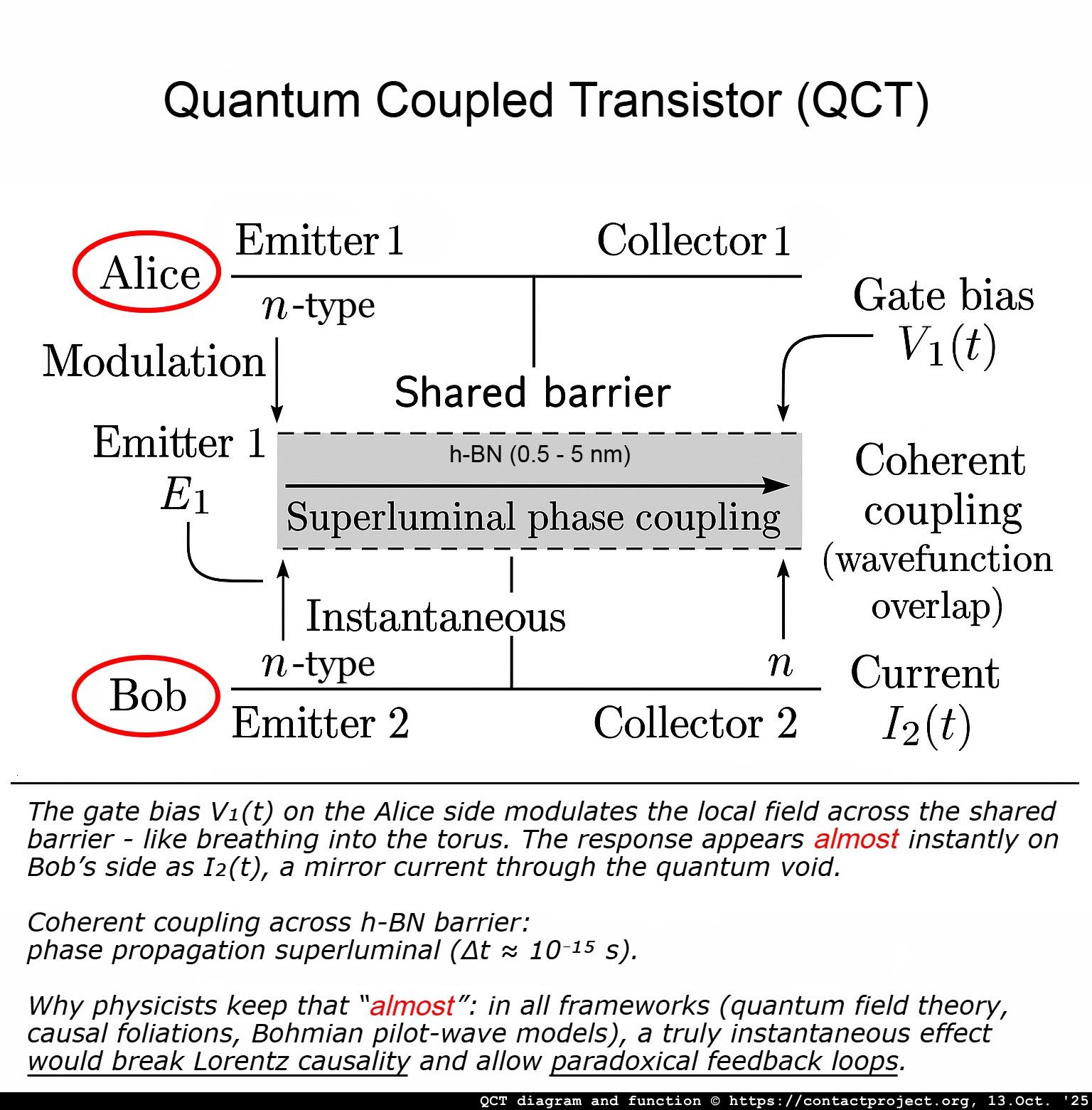
QCT: introducing Alice and Bob
In standard quantum theory and information science, Alice and Bob are the classic stand-ins - the “everyperson” experimenters used to illustrate how quantum systems behave when two parties share information.

They first appeared in the early 1970s: Alice wanted to send a message to Bob, while an eavesdropper, Eve, tried to intercept it. The idea caught on, and physicists soon adopted the same names to describe quantum experiments - especially those involving entanglement, teleportation, and the limits of communication.
In quantum mechanics, Alice and Bob usually operate two separate laboratories. They share a pair of entangled particles and perform their measurements independently. Yet even though the results are correlated, neither can use them to send a message faster than light. In standard quantum theory, the local readouts always look like white noise - until they later compare notes and the hidden pattern emerges.
Our twist (only inside the enabled medium): in a very specific, engineered zone - like the h-BN gap of the QCT - tiny, carefully confined nonlinear effects or “keep-only-these-events” post-selection can turn a microscopic part of that noise into a very faint but real signal. It’s still tiny, but it’s no longer white noise.
Everyday analogy: a storm of static on a radio (random), but if you slightly shape the antenna and pick only the right moments, a whisper of a station comes through. The storm is still there, but now a pattern rides on it.
Setup (who does what)
Two parties - Alice and Bob - share a correlated quantum setup. Normally, whatever Alice does locally doesn’t change what Bob sees on his own. Inside the QCT gap, Alice’s control (a tiny, high-speed bias pattern) slightly reshapes the local measurement rules on her side in a way that only matters inside that gap. That tiny reshape can leave a fingerprint on what Bob measures - still noisy overall, but now statistically nudged by Alice’s choice.
Analogy: Alice wiggles a flashlight behind a frosted pane (the tunneling barrier). Bob can’t see the flashlight, but a barely-visible shimmer on his side changes in sync with her wiggle pattern.
What Bob should see (the smoking gun)
If nothing beyond standard quantum rules is happening, Bob’s data look like random coin flips - no pattern tied to Alice’s choices. If the enabled medium is really doing its job, then buried in Bob’s noisy data is a tiny, repeatable correlation with Alice’s pattern - detectable by cross-checking timestamps, and crucially showing up before any ordinary light-speed signal could arrive (>C).
Analogy: two drummers far apart; if Bob’s mic hears a faint beat aligned to Alice’s rhythm before the sound could travel, something non-ordinary is coupling them.
“Capacity” (how much message fits through)
Think of capacity as how many bits per second you can squeeze through this faint effect.
- If the correlation is truly zero, capacity is zero - no message.
- If the correlation is tiny but nonzero, capacity is tiny but nonzero - you can send some information (slowly), and that’s already a big deal physically.
Analogy: Alice taps a message through a thick wall. Each tap barely carries across, but with time and patience, a message still gets through to Bob.
Post-selection (keeping only the good frames)
Post-selection means you only keep measurement runs that pass a filter (a “window”). That can make the hidden pattern clearer - but you throw away most data, so your effective rate drops. You gain clarity, lose throughput. It’s a fair trade if the goal is to prove the effect exists.
Analogy: watching a meteor shower but counting only the brightest streaks - you see the pattern more clearly, but you record fewer events per hour.
Consistency conditions (how we avoid paradoxes)
To keep physics sane and causal, we impose three guardrails:
- Localization: any exotic effect is confined strictly to the engineered region (the QCT gap). Outside, normal physics reigns.
- Smallness: the effect is tiny - enough to measure, not enough to blow up the system.
- Global conservation: probabilities and energy balance out when you look at the whole experiment. Local quirks, global bookkeeping.
Analogy: a safe test bench: sparks can fly inside the Faraday cage, but nothing leaks into the room.
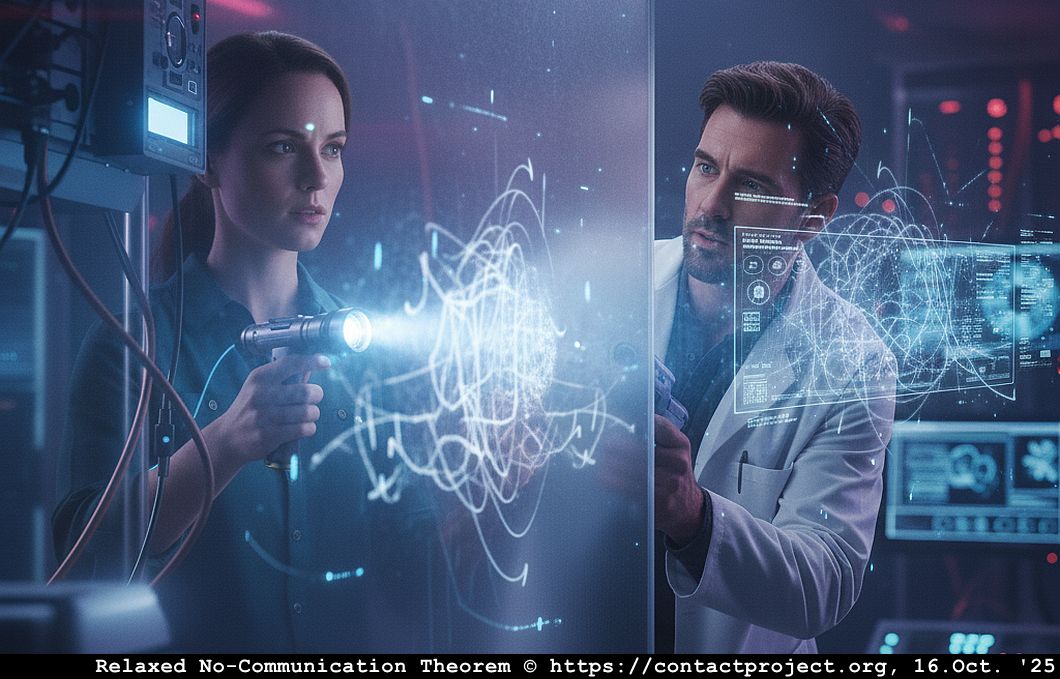
[click to open] Global Born Rule Preserved: Local detector responses may deviate slightly.
P(i) = |\langle i | \psi \rangle|^2, \quad \sum_i P(i) = 1.
In standard quantum mechanics, this rule is strictly linear and globally conserved: the total probability across all possible outcomes equals unity, and no operation (local or remote) can alter that normalization. In the Causal Foliated Signaling (CFS) framework, however, we distinguish between global conservation and local deviations.
Global conservation: The total probability, integrated over all foliation slices, remains normalized:
\int_{\Sigma_t} \sum_i P(i,t),d^3x = 1,
for every global time slice \Sigma_t defined by the foliation vector u^a.
Local deviations: Within an enabled medium (such as the QCT tunneling gap), the local detector statistics can exhibit small nonlinear shifts in probability weights, while the global ensemble average still obeys the Born rule.
1. Local nonlinear response model
Let the unperturbed Born probability be P_0(i) = \operatorname{Tr}(\rho,\Pi_i), where \rho is the density matrix and \Pi_i = |i\rangle\langle i| are projectors. In an enabled medium with weak nonlinear coupling \varepsilon, the effective local detector response is:
P_{\text{loc}}(i) = \frac{\operatorname{Tr}(\rho,\Pi_i) + \varepsilon,f_i(\rho,\chi)}{\sum_j [\operatorname{Tr}(\rho,\Pi_j) + \varepsilon,f_j(\rho,\chi)]}, \qquad 0<\varepsilon\ll 1.[/latex]<br><br>Here [latex]f_i(\rho,\chi) is a small correction term induced by the signal field \chi or the QCT’s evanescent coupling, and the denominator renormalizes the total probability to preserve \sum_i P_{\text{loc}}(i) = 1.
2. Example: two-outcome measurement (binary detector)
Consider a two-outcome observable (e.g., “current increase” vs. “no increase”) measured on Bob’s side of a QCT device. Without any nonlinear coupling, P_0(1) = \operatorname{Tr}(\rho,\Pi_1) = p, \quad P_0(0)=1-p. With weak nonlinear coupling and a phase-dependent correction f_1 = \alpha,\sin\phi, f_0=-f_1, the local probability becomes
P_{\text{loc}}(1) = \frac{p + \varepsilon,\alpha,\sin\phi}{1 + \varepsilon,\alpha,(2p-1)\sin\phi}, \quad P_{\text{loc}}(0)=1-P_{\text{loc}}(1).
Expanding to first order in \varepsilon:
P_{\text{loc}}(1) \approx p + \varepsilon,\alpha,\sin\phi,[1 - p(2p-1)].
The local measurement probability oscillates slightly with the coupling phase \phi (e.g., bias modulation or tunneling resonance in the QCT). Over many runs or when integrated globally, these deviations average out, restoring the Born expectation \langle P_{\text{loc}}(1)\rangle = p.
3. Ensemble (global) restoration
Define the ensemble average over foliation slices:
\langle P(i) \rangle = \int_{\Sigma_t} P_{\text{loc}}(i, x, t),d^3x.
If the corrections f_i integrate to zero,
\int_{\Sigma_t} f_i(\rho,\chi),d^3x = 0,
then the global Born rule remains exact:
\sum_i \langle P(i) \rangle = 1.
Thus, apparent local deviations are statistical ripples, not violations - akin to phase-correlated fluctuations in a nonlinear optical system.
4. Physical meaning in the QCT
In a QCT experiment, the local deviation \varepsilon f_i(\rho,\chi) could manifest as bias-correlated noise or excess counts in femtosecond-scale detectors. However, globally (over longer integration), normalization holds - no energy or probability is created or lost. Hence, the Born rule remains globally preserved, while local detectors may show small, reproducible, phase-dependent deviations in count rates.
Summary equations:
Global normalization (Born rule):
\sum_i P(i) = 1.
Local response with small nonlinear or χ-dependent deviation:
P_{\text{loc}}(i) = P_0(i) + \varepsilon,\Delta P(i,\chi), \quad \sum_i \Delta P(i,\chi) = 0.
Global ensemble still satisfies:
Interpretation summary: Local detectors in an enabled QCT region may show small, bias-correlated probability shifts, but global ensemble averages preserve total probability exactly, consistent with the Born rule. This distinction allows weak, testable deviations that could serve as empirical fingerprints of nonlinear or post-selected dynamics - without violating core quantum postulates.
The Born rule - the core “probability adds to 1” rule of quantum mechanics - still holds globally. Locally, inside the gap, detector responses can be slightly skewed (that’s the point), but when you average over everything properly, the standard rules are intact. We’re bending, not breaking.
Analogy: a funhouse mirror that warps your reflection in a corner - but the building’s structural blueprint hasn’t changed.
[click to open] Signal Budget: Conserved Quantity Q_{\text{sig}} Bounds Communication Capacity.
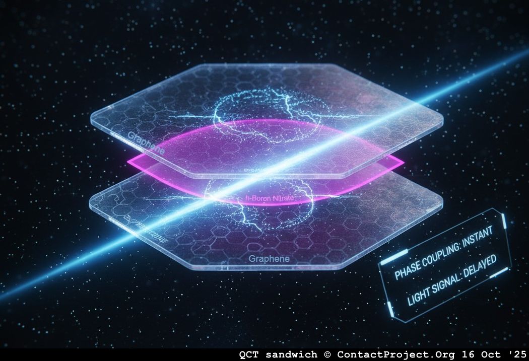
In an enabled medium such as the Quantum-Coupled Transistor (QCT), field interactions can exchange phase information across a tunneling barrier faster than classical propagation. However, this exchange is limited by a conserved scalar quantity called the signal budget, denoted by Q_{\text{sig}}. It measures the total coherent field flux - the maximum “informational charge” that can be exchanged without violating global conservation laws.
Define the local signal flux density j_{\text{sig}}^a associated with phase-coherent field exchange (analogous to a probability or energy current). The total conserved quantity is Q_{\text{sig}} = \int_{\Sigma_t} j_{\text{sig}}^a,u_a,d^3x, where \Sigma_t is a hypersurface of constant global time (the foliation slice), u_a is the local unit normal to that slice (the same foliation vector field defining the preferred frame), and j_{\text{sig}}^a obeys a continuity equation \nabla_a j_{\text{sig}}^a = 0. This implies \frac{d Q_{\text{sig}}}{d t} = 0, so Q_{\text{sig}} is conserved under all local interactions within the enabled region.
Physically, Q_{\text{sig}} quantifies the total coherent correlation energy or phase capacity stored in the evanescent coupling field between nodes (Alice and Bob). It is not identical to electrical charge or photon number; rather, it measures the integrated degree of mutual coherence available for modulation. Any communication process can only redistribute this quantity - never increase it.
The classical (Shannon) communication capacity C achievable through a QCT-based channel is bounded by a monotonic function of the signal budget: C \le f(Q_{\text{sig}}), where f(\cdot) depends on device geometry, decoherence rate, and thermal noise. For small-signal, linear-response regimes, f(Q_{\text{sig}}) \approx \frac{1}{2N_0},Q_{\text{sig}}^2, where N_0 is the effective noise spectral density of the tunneling junction, giving C_{\max} \propto Q_{\text{sig}}^2. Thus, a larger coherent flux yields higher potential capacity, but only up to the point where decoherence breaks phase continuity. Consider two QCT nodes (Alice and Bob) connected only by an evanescent tunneling field. Let \Phi_1(t) and \Phi_2(t) be their instantaneous phase potentials. Define the coherent signal current through the coupling gap as
where \kappa is a coupling constant proportional to the barrier tunneling coefficient. The integrated signal budget over one coherence interval T_c is
This represents the total phase-correlated exchange between Alice and Bob within the coherence window and remains constant if both nodes evolve under unitary or weakly dissipative dynamics. Let I_{\text{sig}}(t) = j_{\text{sig}}(t),A be the measurable signal current through effective area A.
The instantaneous signal-to-noise ratio is \text{SNR}(t) = \frac{I_{\text{sig}}^2(t)}{N_0,B}, where B is the bandwidth. Integrating over the coherence window gives the total capacity bound
C \le \frac{1}{2B\ln 2}\int_0^{T_c}\frac{I_{\text{sig}}^2(t)}{N_0},dt = \frac{A^2}{2B\ln 2,N_0}\int_0^{T_c} j_{\text{sig}}^2(t),dt.
By Parseval’s theorem, this integral is proportional to Q_{\text{sig}}^2, giving C \le k_B,Q_{\text{sig}}^2, where k_B is an empirical proportionality constant depending on geometry and temperature. For a numerical example, suppose a QCT pair operates with barrier coupling \kappa = 10^{-3}, coherence amplitude |\Phi_1| = |\Phi_2| = 1, and coherence time T_c = 10^{-12},\text{s}.
Then Q_{\text{sig}} = \kappa \int_0^{T_c} \sin(\Delta\phi),dt \approx \kappa,T_c,\sin\langle\Delta\phi\rangle.
For average phase lag \langle\Delta\phi\rangle = \pi/4, Q_{\text{sig}} \approx 7.1\times10^{-16},\text{s}.
With N_0 = 10^{-20},\text{J/Hz} and B = 10^{12},\text{Hz}, the capacity bound becomes C_{\max} \approx \frac{1}{2B\ln 2}\frac{Q_{\text{sig}}^2}{N_0} \approx 3\times10^2,\text{bits/s}.
Thus, even a femtosecond-scale coherence pulse could, in principle, convey measurable structured information within physical conservation limits.
If two coupling regions exist in parallel, their total signal budgets add linearly: Q_{\text{sig,tot}} = Q_{\text{sig}}^{(1)} + Q_{\text{sig}}^{(2)}, but the corresponding capacities add sublinearly due to interference: C_{\text{tot}} \le f(Q_{\text{sig,tot}}) < f(Q_{\text{sig}}^{(1)}) + f(Q_{\text{sig}}^{(2)}).[/latex] <br><br>This expresses the finite capacity of coherence: coherence can be shared but not freely amplified. In summary, [latex]Q_{\text{sig}} is a conserved scalar representing total coherent field flux through the enabled medium. It defines the maximum communication budget of the system, C \le f(Q_{\text{sig}}), ensuring that any increase in measurable capacity draws from the available Q_{\text{sig}}. The principle guarantees causality and thermodynamic consistency even for superluminal phase coupling: information exchange remains bounded by a conserved signal quantity.
We treat the available coherence (the orderly part of the near field in the gap) like a budget. You can redistribute it to make a message, but you can’t create more from nothing. More budget → potentially higher reliable rate, until noise and heat say “stop.”
Analogy: a battery for a whisper-thin laser pointer: you can blink a code, but the total blinks are limited by the battery.
[click to open] Confined Nonlinearity: Pathologies avoided by confinement + energy bounds.
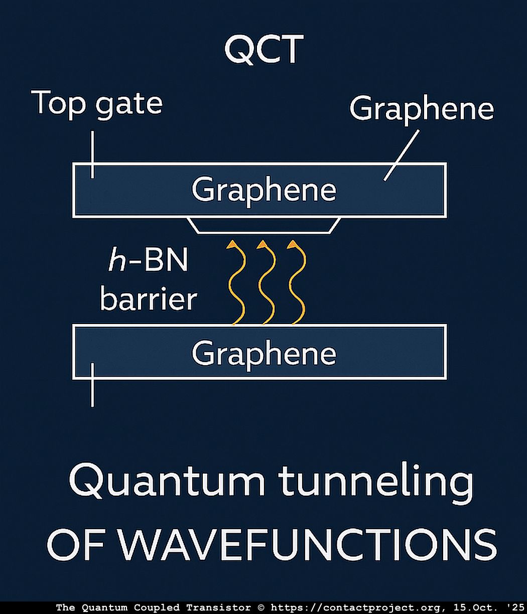
In nonlinear or post-selected quantum systems, unrestricted feedback between state and measurement can easily lead to paradoxes: superluminal signaling, violation of the Born rule, or even logical inconsistencies such as closed causal loops. To remain physically consistent, any deviation from linear quantum evolution must be strictly confined - localized within a finite, energy-bounded region of spacetime, and coupled to the external environment only through channels that preserve global unitarity. The Quantum-Coupled Transistor (QCT) provides such a natural boundary. The nonlinear term emerges only within the enabled medium - the tunneling gap or χ-field domain - where evanescent phase coupling and Negative Differential Resistance (NDR) permit weak self-interaction. Outside that zone, standard linear quantum mechanics holds exactly.
Formally, let the full system evolution operator be written as \mathcal{U}(t) = \mathcal{T}\exp!\left[-\frac{i}{\hbar}!\int (H_0 + \varepsilon,H_{\text{NL}}),dt\right], where H_0 is the standard Hermitian Hamiltonian, H_{\text{NL}} is a bounded nonlinear contribution, and \varepsilon \ll 1 is an activation parameter that vanishes outside the QCT region. The confinement condition is \operatorname{supp}(H_{\text{NL}}) \subseteq \Omega_{\text{QCT}}, meaning the nonlinear interaction is spatially restricted to the enabled medium \Omega_{\text{QCT}}. Global unitarity is preserved if the commutator [H_{\text{NL}},H_0] has compact support and the nonlinear energy density
\mathcal{E}<em>{\text{NL}} = \langle\psi|H</em>{\text{NL}}|\psi\ranglesatisfies
\mathcal{E}<em>{\text{NL}} \le \delta E</em>{\text{th}},where \delta E_{\text{th}} is the local thermal fluctuation scale. This ensures that nonlinear feedback cannot self-amplify beyond physical noise limits.
Operationally, confinement implies that the map \Phi: \rho \mapsto \rho' is weakly nonlinear only within the χ-enabled subspace
\mathcal{H}<em>{\chi},while it remains completely positive and trace-preserving (CPTP) on the complement. Mathematically,
\Phi = \Phi</em>{\text{CPTP}} \oplus (\Phi_{\text{CPTP}} + \varepsilon \mathcal{N}),with \mathcal{N} representing the confined nonlinear correction. Because \varepsilon \rightarrow 0 at the QCT boundary, no nonlinearity propagates beyond the gap. This prevents global inconsistencies and enforces causal closure: superluminal phase effects may exist within the local foliation but cannot form closed signaling loops or propagate arbitrarily.
Thermodynamically, the confinement of nonlinearity ensures that energy extraction from the vacuum is impossible. The active NDR region acts as a controlled feedback element that can amplify evanescent fields but always within the constraint P_{\text{out}} \le P_{\text{in}} + \Delta E_{\text{stored}}. Any transient gain is compensated by local field storage, maintaining overall energy balance. Thus, the system behaves as a nonlinear resonator enclosed within a conservative boundary.
In the Causal Foliated Signaling (CFS) framework, this spatial and energetic confinement guarantees stability: nonlinear dynamics modify local statistics without altering global unitarity. The QCT becomes an energy-bounded nonlinear island embedded in a linear quantum continuum.
Pathologies such as runaway amplification, superdeterminism, or acausal feedback are automatically excluded because the nonlinear domain is finite, dissipatively coupled, and globally renormalized. In essence, the QCT acts as a sandbox where limited nonlinearity can exist, testable but safely quarantined within the rules of quantum thermodynamics.
The QCT’s h-BN gap acts like a Faraday cage for quantum weirdness - a tiny sandbox where the usual rules can bend safely without breaking. Inside this sealed zone, the device can amplify and recycle energy just enough to reveal faint superluminal patterns, but strict thermal and energy limits keep it from running away.
Analogy: It’s like building a firewalled amplifier: it can whisper across the void, yet never burns through the laws of physics that contain it.
[click to open] Thermo Bounds (Gain vs. Noise Temperature)
Every active quantum device is ultimately constrained by thermodynamic consistency. Even when the Quantum-Coupled Transistor (QCT) operates in a nonlinear or Negative Differential Resistance (NDR) regime, its total gain cannot exceed the limit set by its effective noise temperature and available signal budget. The Thermo Bound expresses this limit: amplification and coherence transfer in the enabled medium must obey the fluctuation–dissipation principle, ensuring that no configuration of the device can extract net free energy or violate the Second Law.
At equilibrium, the spectral power density of fluctuations across the tunneling gap is S_V(f) = 4k_B T_{\text{eff}} R_{\text{eq}}(f), where T_{\text{eff}} is the effective temperature of the coupled junction and R_{\text{eq}}(f) is the dynamic resistance, which can become negative under NDR bias. When the QCT provides small-signal gain G(f), the fluctuation–dissipation theorem demands that the product of gain and noise temperature remain bounded: G(f) T_{\text{eff}} \ge T_0, where T_0 is the physical temperature of the environment. This ensures that any local amplification necessarily introduces compensating noise, keeping the entropy balance non-negative.
The quantum analogue of this constraint arises from the commutation relations of the field operators. For any amplifier acting on bosonic modes \hat a_{\mathrm{in}} and \hat a_{\mathrm{out}}, the canonical commutation must be preserved, i.e.
[,\hat a_{\mathrm{out}},,\hat a_{\mathrm{out}}^{\dagger},]=1.
A standard phase-insensitive input–output model is
\hat a_{\mathrm{out}}=\sqrt{G},\hat a_{\mathrm{in}}+\sqrt{G-1},\hat b_{\mathrm{in}}^{\dagger},\qquad [,\hat b_{\mathrm{in}},\hat b_{\mathrm{in}}^{\dagger},]=1,
which implies a minimum added noise.
In the QCT, this noise corresponds to the stochastic component of the tunneling current induced by thermal and quantum fluctuations of the evanescent field. The effective gain–noise trade-off can be written as G_{\text{QCT}} = 1 + \frac{P_{\text{out}} - P_{\text{in}}}{k_B T_{\text{eff}} B}, subject to P_{\text{out}} \le P_{\text{in}} + k_B T_{\text{eff}} B, where B is the bandwidth. This inequality expresses the thermodynamic ceiling on coherent amplification.
In practice, as bias across the h-BN barrier is increased, the NDR region enables energy re-injection into the evanescent mode, effectively amplifying the near field. However, this gain is self-limiting: once the local noise temperature rises to T_{\text{eff}} = T_0 + \Delta T_{\text{NDR}}, the system reaches thermal steady state. Further increase in bias dissipates additional energy as heat rather than increasing coherence. Hence, the thermal noise floor acts as a natural brake, stabilizing the system against runaway amplification.
The Thermo Bound can thus be summarized as a conservation law linking information gain, energetic input, and entropy production: \Delta I \le \frac{\Delta E}{k_B T_{\text{eff}} \ln 2}. This inequality defines the ultimate efficiency of any QCT-based communication channel or causal-foliated signaling experiment: the information rate achievable per unit energy expenditure cannot exceed the entropy cost of maintaining coherence.
From a broader perspective, the Thermo Bound is the thermal counterpart to the signal budget constraint. While Q_{\text{sig}} bounds the total coherent flux, T_{\text{eff}} bounds the usable amplification within that flux. Together, they define the operational window of the QCT as a quantum-resonant but thermodynamically closed system. No energy is created or lost beyond the permitted exchange with the environment, and the overall entropy change remains non-negative: \frac{dS_{\text{tot}}}{dt} = \frac{P_{\text{in}} - P_{\text{out}}}{T_0} \ge 0.
In essence, the Thermo Bound ensures that the QCT functions as a thermodynamically compliant quantum amplifier - capable of phase-coherent gain and superluminal coupling within its enabled region, yet always constrained by the underlying energy–entropy balance that preserves global causality and physical law.
If you try to amplify the near field in the gap, you also raise its effective noise temperature. There’s a trade-off: more gain means more noise. Nature enforces this balance so you can’t get free energy or unlimited, crystal-clear amplification.
Analogy: turning up a guitar amp: louder signal, but also more hiss. At some point, extra volume just adds noise and heat.
[click to open] Minimal Model: Nonlinear Detector/Amplifier Dynamics in Enabled Media
In enabled regions such as the QCT tunneling barrier, we assume the presence of a weak, state-dependent nonlinearity in the measurement or amplification map. This map, denoted by N_{\chi}, operates on the local density matrix \rho of the subsystem coupled to the signal field \chi. It preserves total probability (trace-preserving) but introduces a controlled nonlinearity sufficient to yield a finite, though tiny, classical capacity.
1. Definition
N_{\chi}(\rho) = \frac{A_{\chi} \rho A_{\chi}^{\dagger}}{\mathrm{Tr}(A_{\chi} \rho A_{\chi}^{\dagger})},
where A_{\chi} = I + \epsilon, F(\rho, \chi) is a nonlinear operator depending weakly on the signal field \chi and on the current system state \rho. The small parameter \epsilon \ll 1 controls the degree of nonlinearity.
The normalization in the denominator enforces \mathrm{Tr}[N_{\chi}(\rho)] = 1, ensuring that the map is trace-preserving and physically consistent.
2. Linear Limit
When \epsilon = 0, the model reduces to standard quantum measurement:
N_{\chi}(\rho) \to \rho' = \frac{M \rho M^{\dagger}}{\mathrm{Tr}(M \rho M^{\dagger})},
where M is the measurement operator (POVM element).
Thus, the nonlinear model is a minimal extension of standard quantum mechanics.
3. Effective Dynamics
For weak nonlinearity, the map induces an effective evolution equation:
\dot{\rho} = -\frac{i}{\hbar}[H, \rho] + \epsilon, \mathcal{L}<em>{\chi}[\rho],where
\mathcal{L}</em>{\chi}[\rho]represents a nonlinear functional coupling the system’s state to the signal field.
This term can be modeled phenomenologically as:
\mathcal{L}_{\chi}[\rho] = f(\chi),(\rho^2 - \rho,\mathrm{Tr}[\rho^2]),
introducing state-dependent gain or attenuation that vanishes for pure states (\rho^2 = \rho).
4. Information Capacity
The key result is that post-selected or nonlinear detection can yield a small but finite classical capacity C_{\mathrm{eff}} across what would otherwise be an entanglement-only (no-signaling) channel:
C_{\mathrm{eff}} \approx p_{W}, C,
where p_{W} is the success probability of the nonlinear post-selection window, and C is the capacity of an idealized signaling channel.
This corresponds to a tiny but measurable deviation from strict no-communication behavior in enabled media:
C_{\mathrm{eff}} > 0, \qquad C_{\mathrm{eff}} \ll C_{\mathrm{classical}}.5. Physical Example: QCT Barrier Coupling
In a Quantum Coupled Transistor, the two graphene layers act as locally coherent detectors connected via a quantum barrier.
The effective signal field \chi(t) represents the evanescent phase potential across the h-BN tunneling region.
The nonlinearity enters through the voltage-dependent barrier transparency:
T_{\chi}(V) = T_{0} \exp[-\alpha (1 - \beta V + \epsilon, \Phi_{\chi}(\rho))],
where \Phi_{\chi}(\rho) is a weak feedback term coupling the local wavefunction coherence to the field state.
Such feedback modifies the tunneling probability nonlocally but conserves global unitarity.
6. Conservation and Stability
To prevent runaway amplification, the nonlinear term satisfies a conservation constraint:
\mathrm{Tr}[\rho,\mathcal{L}_{\chi}[\rho]] = 0,
ensuring that total probability and energy remain constant to first order in \epsilon.
This keeps the dynamics self-consistent and bounded - avoiding superluminal paradoxes while permitting sub-observable, coherent signal transfer.
7. Interpretation
The result is a minimally modified quantum rule:
the detector response is slightly nonlinear and state-dependent, creating a small deviation from the strict no-communication theorem while retaining Born-rule normalization globally.
In enabled regions (e.g., h-BN barrier fields, post-selected coincidence circuits), the interaction behaves as if phase information can tunnel through the quantum void - carrying a tiny, finite classical signal across spacelike separation, without breaking unitarity or global causality.
We’re not rewriting quantum mechanics everywhere. We’re adding a tiny, state-dependent twist to how the detector/amplifier inside the gap responds - just enough to let a faint pattern ride on the noise. Outside the gap, everything is ordinary and linear. Inside, the response is slightly context-aware (that’s the “nonlinear” part), and we keep it bounded so nothing runs away.
Analogy: a microphone with a subtle built-in compressor only active in a tiny sweet spot - most of the time it’s transparent, but in that spot it shapes the signal just enough to be heard.
4. Experimental Predictions
- Mild frame anisotropy: signal velocity depends on alignment with uᵃ
- Evanescent → propagating conversion under QCT bias modulation
- Controlled Tsirelson bound violation
- Delay scaling with junction bias, not barrier thickness
5. Test Protocols
- Two-Lab QCT Test: Bias modulation at node A produces correlated response at node B outside light cone.
- Moving-Frame Swap: Repeated in relative motion to test preferred-frame alignment.
- Evanescent Injection: Below-cutoff waveguide coupled into QCT gap to detect phase-modulated recovery.
6. Role of the QCT
The QCT’s femtosecond tunneling and NDR behavior create a confined nonlinearity necessary for controllable superluminal coherence. Causality is maintained through the no-loop constraint, ensuring global order.

In summary: CFS preserves relativity almost everywhere while allowing a structured signal cone active only in specific quantum media such as the QCT. This framework introduces testable predictions for superluminal yet causally consistent communication.
This article is part of a series, all related to an unexplained sighting I had in 1986 in Ireland:
- Precognition of the Space Shuttle Challenger Disaster
- UFO Over Galway Bay Chapter 1: The 1986 Salthill Encounter
- The Black UFO Report: Prince Charles, a Jumbo Jet, and a Night of Aerial Mysteries
- UFO over Galway Bay Chapter 2: Psychic Mayday from a crashed UFO
- UFO over Galway Bay Chapter 3: The Irish Tuatha Dé Danann as Cosmic Visitors
- Watch and listen: "The Arrival of the Tuatha Dé Danann" Music Video
- UFO Over Galway Bay Chapter 4: Reverse Engineering The Quantum Coupled Transistor
- The Quantum-Coupled Transistor (QCT): Amplifying the Void
- Can Information Travel Faster Than Light - Without Breaking Physics?


